Predicting Auto Insurance Pure Premium
Introduction
The Kangaroo Insurance Case competition organized by Travelers Insurance asked the Data Science community at UMass and UConn to predict claim costs for auto insurance policies. The 50+ teams were given an anonymized dataset with about 20k training samples. The challenge was to get predictions with the highest gini coefficient on the hold set. Our team consisting of Rajarshi Roychowdhury, Aruni Roychowdhury and Neil Patel ranked second (2nd) in a head-to-head race at the end with a final gini coefficient of 0.229
Business problem
You work for Kangaroo Auto Insurance Company, an Australian company. Your business partner, who is not familiar with statistics at all, would like you to create a rating plan based on the historical auto claim data. Your business partner is concerned about segmentation as well as competitiveness, as there are several other competitors in the market. For this case competition, your group’s task is to provide a method for predicting the claim cost for each policy and to convince your business partner that your predictions will work well.
Data Description
The Kangaroo data set is based on one-year vehicle insurance policies from 2004 to 2005. The data is split into two parts: training and validation set. The actual competition had a third set (hold set) on which teams were scored.

Variable information in the data:
- ID: policy key
- Veh_value: market value of the vehicle in $10,000’s
- Veh_body: Type of vehicles
- Veh_age: Age of vehicles (1=youngest, 4=oldest)
- Gender: Gender of driver
- Area: Driving area of residence
- Dr_age: Driver’s age category from young (1) to old (6)
- Exposure: The basic unit of risk underlying an insurance premium
- Claim_ind: Indicator of claim (0=no, 1=yes)
- Claim_counts: The number of claims
- Claim_cost: Claim amount
What is the actual end goal?
Auto Insurances must be priced to reflect the provider’s risk exposure. Thus, the pricing of an insurance policy depends on the underlying risk exposure of the insured. In this example, we are calculating ‘Pure Premium’, which is the average loss per exposure. PP = Frequency * Severity = loss $ / exposure. This is what a company would charge for a policy if not accounting for expenses and profit.
The model results are not evaluated on accuracy, but on the Gini index.
Approaching the problem
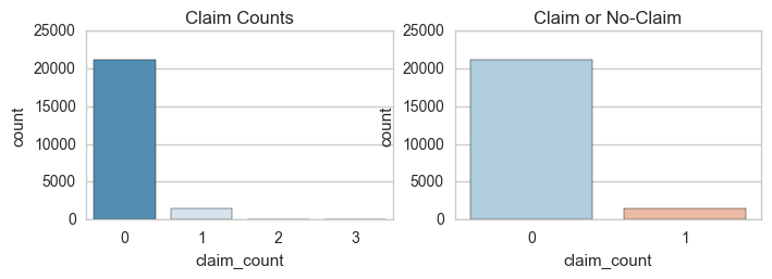
After some basic EDA, it was observed that the data was highly skewed. Less than 7% of the data points had any claims, and the vast majority of our data had no claims. It was further observed that less than .4% of the data had greater than a single claim. So, we converted the numeric claim_count variable into a binary feature (0=no claim, 1=claim).
df['claim_count'] = df['claim_count'].apply(lambda x:1 if x>0 else 0)

1. Predict Claim Probability using Logistic Regression
First, we train a Logistic Regression model to calculate the probabilities of having a claim on the test set. Since the number of negative labeled values far exceed the positive labeled values, we use bagging, i.e. create bootstrap samples of the data with equal number of positive and negative classes. We create 1000 such samples, train a logistic regression model on each of them, and finally use majority voting on the resulting ensemble of classifiers.
from sklearn.linear_model import LogisticRegression
logmodel = LogisticRegression(C=1000, class_weight='balanced')

n=10 #Number of models to run
for i in range (0,n):
    X_train_neg = X_train.loc[np.random.choice(df[df['claim_count']==0].index, 3000, replace = False)]
    X_train_pos = X_train.loc[np.random.choice(df[df['claim_count']==1].index, 3000, replace = True)]
    X_train = pd.concat([X_train_pos,X_train_neg], ignore_index=True)

    y_train = X_train['claim_count']
    X_train.drop('claim_count', axis=1,inplace=True)

    #Fit the Logistic Regression Model
    logmodel.fit(X_train,y_train)
    y_test['pred'] = y_test['pred'] + logmodel.predict(X_test)

#Take Vote
y_test['pred'] = y_test['pred'].apply(lambda x:1 if x>=5 else 0)

from sklearn.metrics import classification_report
print(classification_report(y_test['claim_count'],y_test['pred']))
Using the trained Logistic Regression model, we calculate z =(P(claim)/P(no-claim))**r. The exponent r controls the “inequality”. Thus higher values (>1) get higher, lower values (<1) get lowered.
2. Predict Claim Value using Gradient Boosted Trees (XGBoost)
To predict claim values, we trained on rows which had at least 1 claim. XGBoost dominates structured or tabular datasets on classification and regression predictive modeling problems, and is becoming the tool of choice for such problems.
X_train_regress = df[df['claim_count']>0].copy()
y_train_regress = np.log(df[df['claim_count']>0]['claim_cost'])

#Implement XGBoost for regression
import xgboost as xgb
num_round = 10

T_train_xgb = xgb.DMatrix(X_train_regress, y_train_regress)
params = {"objective": "reg:linear"}
gbm = xgb.train(dtrain=T_train_xgb,params=params)
predictions = gbm.predict(xgb.DMatrix(X_test))
predicted_claim_cost=[np.exp(p) for p in predictions]
Final claim cost = z * predicted_claim_cost
3. Heuristic factors to boost inequality
Finally, we use manual heuristic factors that we’ve chosen for maximum differentiating ability to increase the inequality in our predicted claim costs. Remember, we are not striving for accuracy, but rather aiming for higher gini coefficient.
Example of Factor Calculation for Area = ‘A’:
In Area ‘A’, say there are 2 claims for 10 non-claims (2/10).
In all other Areas, say there is 1 claim for 20 non-claims (1/20).
Then factor(Area:‘A’) = (2/10)/(1/20) = 4“If you stay in Area A, your claim cost gets bumped up by a factor of 4”
4. Combining with a GLM based model
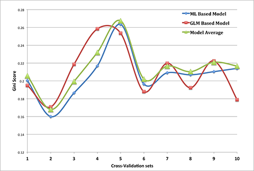
We created a parallel GLM based model to predict claim costs. We used a simple model ensembling technique to combine predictions from both ML based and GLM based models to generate our final predictions. The model stacking was primarily done to reduce variance and introduce better generalizability in our final model. The stacked model outperforms each of the individual models due to its low variance and ability to highlight each model where it performs better.

